
Foundation models like Llama 3, Mistral, and open-weight transformer architectures arrive out of the box with broad linguistic capabilities and extensive general knowledge.
However, when deployed in production, off-the-shelf base models often struggle with domain-specific vocabularies, strict JSON output schemas, proprietary business logic, and deterministic response styles.
While prompt engineering and Retrieval-Augmented Generation (RAG) provide runtime context, they do not fundamentally alter how an artificial intelligence model reasons or structures its outputs.
This is where model fine-tuning comes into play. For software engineers, fine-tuning represents the bridge between a generic pre-trained checkpoint and a specialized, reliable system component.
This guide breaks down how large language model (LLM) fine-tuning works under the hood, compares full fine-tuning with parameter-efficient techniques like LoRA and QLoRA, details dataset preparation, and walks through a complete implementation using the Hugging Face ecosystem.
What Is AI Model Fine-Tuning?
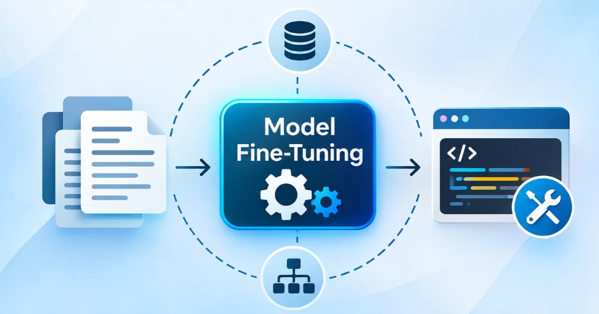
Fine-tuning is the process of taking a pre-trained language model already trained on terabytes of raw text via self-supervised learning and performing additional gradient updates on a curated, domain-specific dataset.
+-----------------------------------------------------------------------+
| Phase 1: Pre-Training (Massive Compute & Web Scale Corpora)          |
| Raw Text -> Next-Token Prediction -> Base Model (e.g., Llama 3 Base)  |
+-----------------------------------------------------------------------+
                                   |
                                   v
+-----------------------------------------------------------------------+
| Phase 2: Supervised Fine-Tuning (SFT) (Curated Pairs & Modest Compute) |
| Prompt-Response Pairs -> Cross-Entropy Loss -> Specialized Task Model  |
+-----------------------------------------------------------------------+
Instead of learning grammar, syntax, and foundational facts from scratch, the model adapts its internal weight representations to specialize in specific downstream tasks, such as:
- Generating valid domain-specific code (e.g., custom DSLs, framework-specific boilerplate).
- Adhering strictly to structured formats (e.g., JSON schemas, XML feeds) without hallucinated wrapper text.
- Embodying a consistent brand tone, technical voice, or deterministic conversational style.
- Executing text classification, entity extraction, or structured summarization without bloated system prompts.
Fine-tuning is fundamentally distinct from Retrieval-Augmented Generation (RAG). While RAG acts as an open-book lookup providing dynamic reference material in the prompt context, fine-tuning acts as internalized habit formation, modifying how the model processes information and articulates answers.
How Does Fine-Tuning Work Under the Hood?
Most modern large language models are decoder-only autoregressive transformers. Understanding how fine-tuning alters these models requires looking at the loss function, tokenization, and parameter optimization mechanics.
1. The Pre-Training Foundation
During pre-training, the model minimizes cross-entropy loss across an objective known as Causal Language Modeling (CLM). Given a sequence of tokens $x = (x_1, x_2, \dots, x_T)$, the model maximizes the likelihood of predicting the next token:
$$\mathcal{L}_{\text{CLM}}(\Theta) = -\sum_{t=1}^{T} \log P(x_t \mid x_1, x_2, \dots, x_{t-1}; \Theta)$$
Where $\Theta$ represents the total weight parameters of the network.
2. Supervised Fine-Tuning (SFT)
In Supervised Fine-Tuning, the training dataset shifts from arbitrary unlabelled text to structured prompt-completion pairs $(X, Y)$. Here, $X = (x_1, \dots, x_n)$ represents the user prompt or instruction, and $Y = (y_1, \dots, y_m)$ represents the target completion.
During training, both $X$ and $Y$ are concatenated and passed through the network, but loss is computed exclusively on the target tokens $Y$. The input tokens $X$ are masked using label indices set to -100 (the default ignore_index in PyTorch’s CrossEntropyLoss).
This ensures that the model is penalized only for mistakes made while generating the response, rather than being forced to memorize or reconstruct the user prompt.
Token Sequence:  [BOS]  Summarize:  The  server  failed.  [SEP]  Hardware  error.  [EOS]
Loss Target:     -100   -100        -100 -100    -100     -100   Hardware  error.  [EOS]
Mask Status:     <------------- MASKED OUT -------------> <--- GRADIENT COMPUTED --->
Full Fine-Tuning vs. Parameter-Efficient Fine-Tuning (PEFT)
Historically, adapting a neural network involved updating all parameters $\Theta$. For modern models spanning 7 billion to 70 billion parameters, this approach presents steep memory and infrastructure bottlenecks.
| Metric / Dimension | Full Fine-Tuning | Parameter-Efficient Fine-Tuning (PEFT / LoRA) |
| Trainable Parameters | 100% of network weights | Typically 0.1% to 2.0% of network weights |
| VRAM Footprint (7B Model) | ~80 GB – 120 GB (Requires A100/H100 GPUs) | ~16 GB – 24 GB (Feasible on RTX 3090/4090 or T4/A10G) |
| Optimizer Memory | Stores FP32 states for all weights | Stores states only for low-rank adapter matrices |
| Checkpoint Storage | 14 GB – 28 GB per fine-tuned variation | 20 MB – 200 MB per adapter artifact |
| Catastrophic Forgetting | High risk without balanced regularization | Substantially lower; base weights remain frozen |
| Multi-Tenant Serving | Requires dedicated GPU memory per model | Single base model in VRAM; dynamic adapter swapping |
The Math Behind Memory Overhead in Full Fine-Tuning
When updating model parameters using optimizers like AdamW, VRAM consumption extends far beyond the static size of the model weights:
- Model Weights: A 7-billion parameter model in 16-bit precision (FP16 or BF16) requires $7 \times 2 = 14\text{ GB}$ of memory.
- Gradients: Gradients stored in 16-bit require another 14 GB.
- Optimizer States: AdamW tracks both the first moment (momentum) and second moment (variance) in full 32-bit float precision ($4\text{ bytes} \times 2 = 8\text{ bytes}$ per parameter), requiring $7 \times 8 = 56\text{ GB}$.
- Activations & Buffers: Forward pass activation tensors scale with batch size and context window length.
Consequently, full fine-tuning of an entry-level 7B model demands roughly 80 GB to 100 GB of addressable VRAM, requiring multi-GPU distributed strategies such as Fully Sharded Data Parallel (FSDP) or DeepSpeed ZeRO.
Deep Dive: LoRA and QLoRA Mechanics
To eliminate the hardware constraints of full fine-tuning, researchers introduced low-rank adaptation techniques that modify parameter behavior without updating the original model weights.
1. LoRA (Low-Rank Adaptation)
Introduced by Hu et al. (2021), LoRA hypothesizes that the weight updates ($\Delta W$) during model adaptation have a low “intrinsic dimension.”
Instead of updating a full-rank linear layer weight matrix $W_0 \in \mathbb{R}^{d \times k}$, LoRA freezes $W_0$ entirely and decomposes the update matrix $\Delta W$ into two low-rank matrices, $A$ and $B$:
$$\Delta W = B \cdot A$$
Where:
- $B \in \mathbb{R}^{d \times r}$
- $A \in \mathbb{R}^{r \times k}$
- The rank $r$ satisfies $r \ll \min(d, k)$ (common choices are $r \in \{8, 16, 32, 64\}$).
          Output h = W0(x) + (alpha / r) * B(A(x))
                          ^
                          |
             +------------+------------+
             |                         |
     Frozen Weight (W0)        Low-Rank Adapter (B * A)
       [d x k Matrix]             B: [d x r] (Zero init)
             |                    A: [r x k] (Gaussian init)
             |                         ^
             +------------+------------+
                          |
                       Input x
During forward inference, the modified computation evaluates as:
$$h = W_0 x + \Delta W x = W_0 x + \frac{\alpha}{r} (B A x)$$
- Matrix $A$ is initialized using a Gaussian distribution, and matrix $B$ is initialized to zero, ensuring that $\Delta W = 0$ at the start of training.
- The scalar scaling factor $\frac{\alpha}{r}$ stabilizes optimization when experimenting with different rank values $r$.
- Inference Efficiency: For production deployment, $\Delta W = \frac{\alpha}{r} (B A)$ can be mathematically merged directly into $W_0$, introducing zero additional inference latency.
2. QLoRA (Quantized Low-Rank Adaptation)
Introduced by Dettmers et al. (2023), QLoRA pushes memory efficiency further by quantizing the frozen base model to 4-bit precision while retaining 16-bit trainable adapters. QLoRA introduces three foundational innovations:
- NF4 (NormalFloat 4): An information-theoretically optimal quantile quantization data type for normally distributed neural network weights.
- Double Quantization (DQ): Quantizes the quantization constants themselves, reducing memory consumption by roughly 0.37 bits per parameter.
- Paged Optimizers: Uses CUDA Unified Memory to automatically page optimizer memory allocations between GPU VRAM and CPU RAM during gradient checkpoints, preventing out-of-memory (OOM) crashes on large sequence lengths.
Through QLoRA, developers can fine-tune a 7B or 13B parameter model on a single workstation GPU equipped with 16 GB to 24 GB of VRAM.
Preparing Training Data for Instruction Fine-Tuning
Model output quality depends directly on the quality, balance, and format of the dataset. Fine-tuning models on noisy, repetitive, or malformed examples results in degraded conversational ability and hallucinated syntax.
1. Structural Formatting: Standard JSONL Formats
Instruction datasets are commonly structured as line-delimited JSON (.jsonl). Two main schema conventions dominate modern tooling:
The Alpaca Format (Instruction, Input, Output)
Best suited for direct single-turn execution tasks:
JSON
{"instruction": "Extract the HTTP status code and message.", "input": "Error: 404 Not Found at /api/v1/auth", "output": "{\"status\": 404, \"message\": \"Not Found\"}"}
The OpenAI / ChatML Conversational Format
Standard for multi-turn conversational agents, supported natively by Hugging Face tokenizers via Jinja templates:
JSON
{
  "messages": [
    {"role": "system", "content": "You are a backend engineering assistant. Respond strictly in valid JSON."},
    {"role": "user", "content": "Generate a database schema for a user profile table."},
    {"role": "assistant", "content": "{\"table\": \"users\", \"columns\": [{\"name\": \"id\", \"type\": \"uuid\", \"primary_key\": true}, {\"name\": \"email\", \"type\": \"varchar(255)\", \"unique\": true}]}"}
  ]
}
2. Formatting Using Chat Templates
Modern Hugging Face tokenizers provide an apply_chat_template utility. This injects the exact control tokens (such as <|im_start|>, <|start_header_id|>, or [INST]) that the target model was trained to interpret:
Python
from transformers import AutoTokenizer

tokenizer = AutoTokenizer.from_pretrained("meta-llama/Meta-Llama-3-8B-Instruct")

formatted_prompt = tokenizer.apply_chat_template(
    messages,
    tokenize=False,
    add_generation_prompt=False
)
Step-by-Step Implementation with Hugging Face
The following workflow demonstrates fine-tuning a base model using PyTorch, Transformers, PEFT, BitsAndBytes, and the TRL (Transformer Reinforcement Learning) library.
1. Environment Setup
Install the necessary dependencies via pip:
Bash
pip install torch transformers peft bitsandbytes datasets trl accelerate
2. Complete Python Fine-Tuning Script
This script configures 4-bit QLoRA, mounts low-rank adapters to the attention projection layers, formats the data, and runs training using SFTTrainer.
Python
import torch
from datasets import load_dataset
from transformers import (
    AutoModelForCausalLM,
    AutoTokenizer,
    BitsAndBytesConfig,
)
from peft import LoraConfig, get_peft_model, prepare_model_for_kbit_training
from trl import SFTTrainer, SFTConfig

# 1. Define Model Identifiers
MODEL_ID = "mistralai/Mistral-7B-v0.1"
OUTPUT_DIR = "./results_mistral_adapter"

# 2. Configure 4-bit Quantization (QLoRA)
bnb_config = BitsAndBytesConfig(
    load_in_4bit=True,
    bnb_4bit_quant_type="nf4",
    bnb_4bit_compute_dtype=torch.bfloat16,
    bnb_4bit_use_double_quant=True,
)

# 3. Load Tokenizer & Quantized Model
tokenizer = AutoTokenizer.from_pretrained(MODEL_ID, use_fast=True)
tokenizer.pad_token = tokenizer.eos_token
tokenizer.padding_side = "right"

model = AutoModelForCausalLM.from_pretrained(
    MODEL_ID,
    quantization_config=bnb_config,
    device_map="auto"
)

# 4. Prepare Model for Low-Precision Training
model = prepare_model_for_kbit_training(model)

# 5. Define LoRA Hyperparameters
peft_config = LoraConfig(
    r=16,                           # Bottleneck rank dimension
    lora_alpha=32,                  # Scaling factor
    target_modules=[                # Apply adapters to self-attention layers
        "q_proj",
        "k_proj",
        "v_proj",
        "o_proj"
    ],
    lora_dropout=0.05,
    bias="none",
    task_type="CAUSAL_LM"
)

model = get_peft_model(model, peft_config)

# 6. Load Sample Dataset
# Expects a dataset containing formatted text fields or conversational columns
dataset = load_dataset("philschmid/dolly-15k-oai-style", split="train[:1000]")

# 7. Configure SFT Training Parameters
training_args = SFTConfig(
    output_dir=OUTPUT_DIR,
    num_train_epochs=3,
    per_device_train_batch_size=4,
    gradient_accumulation_steps=4,
    optim="paged_adamw_8bit",
    logging_steps=10,
    learning_rate=2e-4,
    fp16=False,
    bf16=True,                      # Use BF16 on Ampere or newer GPUs
    max_seq_length=512,
    warmup_ratio=0.03,
    lr_scheduler_type="cosine",
    save_strategy="epoch",
)

# 8. Initialize Supervised Fine-Tuning Trainer
trainer = SFTTrainer(
    model=model,
    train_dataset=dataset,
    peft_config=peft_config,
    processing_class=tokenizer,
    args=training_args,
)

# 9. Execute Training Run
trainer.train()

# 10. Persist LoRA Adapter Weights
trainer.model.save_pretrained(OUTPUT_DIR)
tokenizer.save_pretrained(OUTPUT_DIR)
3. Merging Adapters for Low-Latency Serving
To serve the fine-tuned model via deployment frameworks like vLLM, or when running open-source models locally through Ollama or llama.cpp, merge the low-rank adapter weights back into the unquantized base weights to eliminate runtime projection latency.
Python
import torch
from peft import PeftModel
from transformers import AutoModelForCausalLM, AutoTokenizer

BASE_MODEL = "mistralai/Mistral-7B-v0.1"
ADAPTER_PATH = "./results_mistral_adapter"
EXPORT_PATH = "./merged_model"

# Load base model in FP16 (Do NOT quantize when merging)
base_model = AutoModelForCausalLM.from_pretrained(
    BASE_MODEL,
    return_dict=True,
    torch_dtype=torch.float16,
    device_map="cpu",
)

# Mount adapter weights
model = PeftModel.from_pretrained(base_model, ADAPTER_PATH)

# Mathematically fuse W_merged = W_0 + (alpha/r) * (B * A)
merged_model = model.merge_and_unload()

# Export standalone model weights
merged_model.save_pretrained(EXPORT_PATH)
tokenizer = AutoTokenizer.from_pretrained(BASE_MODEL)
tokenizer.save_pretrained(EXPORT_PATH)
Real-World Developer Applications
Fine-tuning is most effective when treating an LLM as a specialized execution engine rather than a general-purpose conversational partner:
- Strict Structured Schema Enforcement: While basic prompt tuning suffices for casual queries, developers engineering autonomous AI agent architectures frequently encounter hallucinated tool arguments and malformed schemas when relying on system prompts alone. Fine-tuning solves this by baking schema compliance directly into the model’s weights.
- Domain-Specific Language (DSL) Translation: Converting natural language directly into internal enterprise query formats, Kubernetes manifests, or custom SQL dialects that do not exist within public GitHub training distributions.
- Latency and Token Optimization: Rather than passing a 2,000-token system prompt containing few-shot examples on every API invocation, fine-tuning embeds the expected behavioral patterns directly into the weights, significantly reducing input token volume, reducing inference latency, and cutting API costs.
- Edge Deployment and Model Distillation: Small models (1B to 3B parameters) can be fine-tuned using high-quality synthetic data generated by larger models (e.g., Llama 3 70B). This produces lightweight models that run locally on mobile devices or edge servers while maintaining high performance on focused tasks.
Benefits, Limitations, and Technical Challenges
Adopting fine-tuning in production software requires evaluating its trade-offs against prompt engineering and RAG.
Benefits
- Consistent Behavior: Enforces style, tone, and functional syntax reliably across millions of inferences.
- Reduced Prompt Overhead: Removes the need to pass multi-shot examples inside prompt contexts, maximizing remaining context capacity for dynamic inputs.
- Operational Sovereignty: Retains full ownership of model weights on self-hosted infrastructure, avoiding third-party API rate limits, provider deprecations, and privacy concerns.
Limitations and Challenges
- Catastrophic Forgetting: Over-tuning a model on narrow datasets can degrade its general reasoning, mathematics, or instruction-following capabilities.
- Stale Knowledge Boundaries: Fine-tuning is an ineffective mechanism for injecting factual, fast-changing knowledge (e.g., today’s stock prices or updated API documentation). Knowledge is best retrieved dynamically via RAG.
- Evaluation Bottlenecks: Evaluating conversational fine-tunes is non-trivial. Developers must build rigorous programmatic evaluation suites using benchmark metrics (e.g., ROUGE, BLEU, exact schema match) or LLM-as-a-judge pipelines.
- Dataset Quality Bottlenecks: Training on 500 clean, meticulously reviewed examples consistently outperforms fine-tuning on 50,000 ambiguous, noisy, or synthetic records.
Frequently Asked Questions (FAQ)
1. When should I choose Fine-Tuning over RAG?
Use RAG when your primary challenge is dynamic, factual data access (e.g., internal documentation, live customer records, knowledge bases that update daily). Use Fine-Tuning when your challenge is format, style, domain syntax, or deterministic execution (e.g., writing valid Cypher queries, enforcing JSON schemas, adopting a brand voice). For enterprise AI architectures, both patterns are frequently combined: fine-tuning teaches the model how to articulate, while RAG provides what to articulate.
2. Can I run LoRA fine-tuning on a standard developer laptop?
Running LoRA on Apple Silicon (M-series chips) is supported through libraries like Apple’s MLX. For Linux/Windows environments, running QLoRA on a 7B parameter model requires an NVIDIA GPU with at least 12 GB to 16 GB of dedicated VRAM (e.g., RTX 3060/4060 or higher). Training without a CUDA-compatible GPU using pure CPU execution is impractically slow for production-scale models.
3. How many training examples are needed for effective SFT?
For narrow, structured tasks (e.g., formatting data into a fixed JSON layout or classifying developer error logs), significant behavioral alignment can be achieved with as few as 500 to 2,000 high-quality, diverse examples. Broad instruction following or complex coding adaptations typically require tens of thousands of verified instances.
4. What is the difference between LoRA rank ($r$) and LoRA alpha ($\alpha$)?
The rank ($r$) defines the inner dimension of the low-rank matrices and dictates the parameter capacity of the adapter; a higher rank allows the adapter to capture more complex behavioral changes at the cost of higher memory usage.
The alpha ($\alpha$) parameter is a constant scaling factor applied to the adapter weight updates ($\frac{\alpha}{r}$). A common rule of thumb is to set $\alpha = 2 \times r$.
Conclusion
Fine-tuning has transitioned from an expensive, research-grade task to an accessible developer optimization workflow. Parameter-efficient fine-tuning methods particularly LoRA and QLoRA allow engineering teams to adapt state-of-the-art open-weight models to custom domains on standard workstation hardware.
By understanding how supervised fine-tuning modifies loss calculation, formatting datasets to align with native tokenizer chat templates, and leveraging the Hugging Face PEFT and TRL ecosystems, developers can build deterministic, high-efficiency AI components tailored to their production software architectures.